
Introduction
In this project we will be discussing how to use a CNN (Convolutional Neural Network) and Transfer Learning as methods for making a dog breed classifier. Welcome to the dog breed classifier in a suppervised learning way.
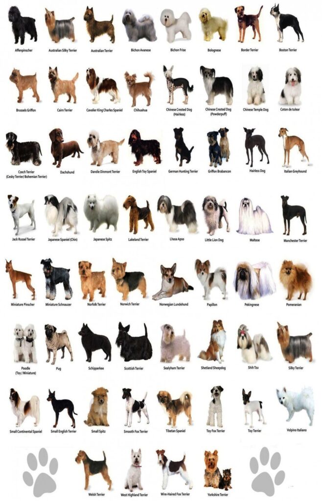
Explaining more about the goal, the task is very simple, given an image of a dog, your algorithm will identify an estimate of the canine’s breed. If supplied an image of a human, the code will identify the resembling dog breed. The dataset consists of 8351 total dog images divided in 133 classes.
CNNs are pretty common type of neural networks and you will find it usefull for many tasks, specially in computer vision demanding applications due to its effectiveness in results. In the end, you could use this model to make a real web application to feed an image and make predictions of the breed of the dog or breed similarity to a human.
Our project is based practically on Tensorflow / Keras libraries and other supported packages.
You can get the project from here.
The Problem
As a Data Scientist you are given the task in develop an algorithm that will be part of a mobile or an web app, this app will be fed with an image.
- If the image is originally a dog image and it is detected will estimate the dog breed.
- If the image is originally an human face image, and it is detected, it will provide the estimated dog breed.
- On the other hand, if there is no human or dog detection it will output an error.
Remember, no algorithm is perfect and in some cases there probably will be bad predictions. But we will discuss it later.
Metric
Accuracy is an easy metric to summarize the result [4]. Actually is the rate of correct predictions vs number of predictions, that is the reason it is so popular. This is a good metric if your dataset is balanced. For imbalanced datasets this metric will not be a good metric to validate our findings/results.
There is a stretch correlation between Error Rate and Accuracy
- Accuracy = 1 – Error Rate
- Error Rate = 1 – Accuracy
Other metric that we could use is a confusion matrix, it is very descriptive and also very informative for more insights of the prediction and mistakes of your model.
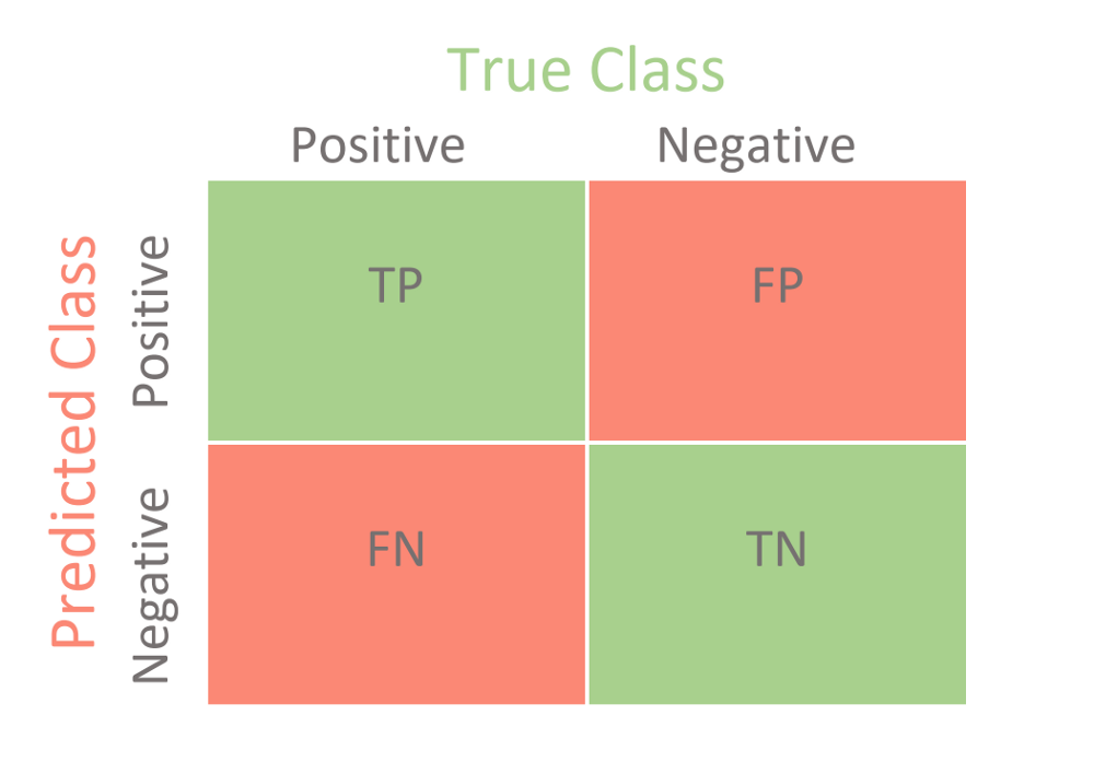
We can calculate the accuracy from that matrix and the error rate:
- Accuracy = (TP + TN)/(TP + FN + FP + TN)
- Error Rate = (FP + FN)/(TP + FN + FP + TN)
OK, back to the problem itself. Because the dataset is an imbalanced dataset (see figure 2 below) and because the distribution of examples in the training dataset across the classes are not equal, in this case, a skew or severe skew in the dataset give us an unreliable measurement of model performance.
In the end, intuition of high accuracy for imbalanced class classifications would be wrong for imbalanced class.
Understanding the Dataset
We will first load the dataset of dogs and humans at first. As usual we first clean the data, but in this situation, the image dataset was curated by the provider. Below you will see the table that ensembles the information of the dog dataset and human dataset and a figure that ensembles the distribution of the full set of images in the dataset
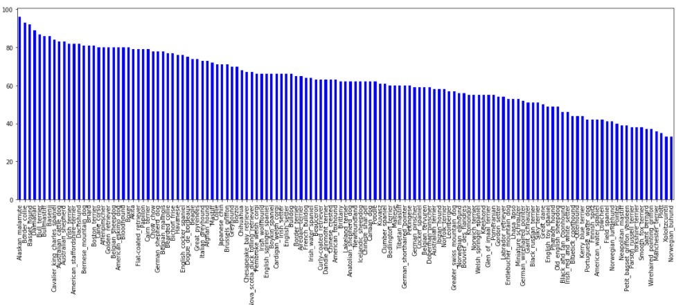
Table 1. Executive Resume of the Datasets
| Dataset | Train Images | Validation Images | Test Images | Total Images |
| Dogs | 6680 | 835 | 836 | 8351 |
| Human | – | – | – | 13233 |
Detecting Faces and Humans
For detecting humans first, we will use another library called OpenCV. OpenCV is a well known library for computer vision. It is more related to computer vision and image processing but people think that is a deep learning library, and it is not, it just have pipeliners and function blocks to load, feed and get the output of a neural network.
For this case, we will use a built in pre-trainded face detector called Haar Cascades[1], specially for frontal faces.
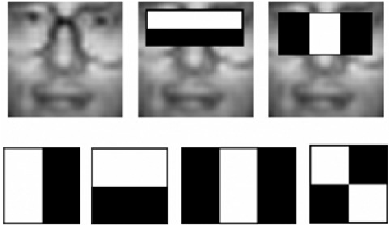
This image is from the paper published in 2001 called, Rapid Object Detection using a Boosted Cascade of Simple Features, a short name of the method is the Viola-Jones detector due to the name of its creators and where one of the first methods of object detection.
This method will slide a window across our image in multiple scales and computed with the quadrature features that you see above (edge features, line features and four-rectangle features), when mixing it, the regional context of importance get us the detection of the face.
Remember that those methods like haar-cascades are old methods and now we have surpassed the accuracy, also, one thing to note is that we need to feed to the detector a gray image, that is because on the old days was the best way to process because the memory and computer resources.
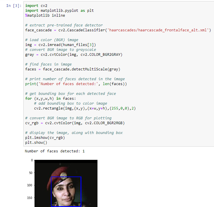
Now that we have a way to detect a face, let’s write a function to help us to detect if is a human present or not. That is very easy to achieve, because the haar cascade detector will give us that information directly.

As we wrote the human detector, let’s see the performance of the algorithm comparing two subsets of 100 images of dogs and 100 images of humans. The result was:
- Percentage of Humans in Humans subset = 100%
- Percentage of Humans in Dogs subset = 11%
The result denotes that our algorithm fails a little of the preffered goal (100% humans, 0% Dogs)
Detecting Dogs
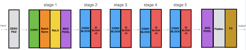
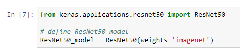
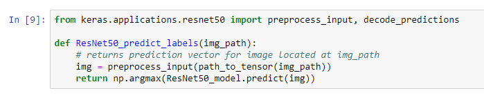
Now we will start using CNNs, basically one based on the ResNet-50 model. Resnet-50 [2] is a popular Deep Learning Model very common in the deep learning world and was the winner on the ImageNet competition in 2015 with an error rate of 3.57% [3].
First of all we must import the resnet model. Fortunatelly, keras has built in functions to call the model in a easy way.
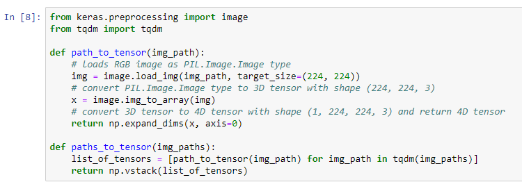
For the information preprocessing lets remember that Keras needs a 4D array, called tensor, to do all it processes. This 4D array is described as below:
- number of samples
- rows
- columns
- channels
On this case the tensor is a (1, 224, 224, 3) that ensembles just one image. Just Remember that the first number of the tensor is related to the number of samples and the rest of the shape of the image.
As we see, first we need to preprocess the image, loading it as a BGR image by reordering the channels. All pretrained models have a normalized RGB pixel that must be substracted, this information is known by the model provider, in the case of Resnet is [103.939, 116.779, 123.68]. So where those values comes from? Those are calculated over the dataset itself, in this case, ResNet.
We can then get the image, preprocess and feed directly to the model to predict the ocurrences, but in the end we will need only the maximun of the occurrences
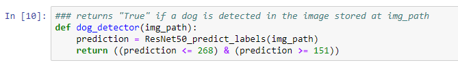
For writing a dog detector we only use part of the dictionary, labels 151 to 268 refering from Chihuahua up to Mexican Hairless.
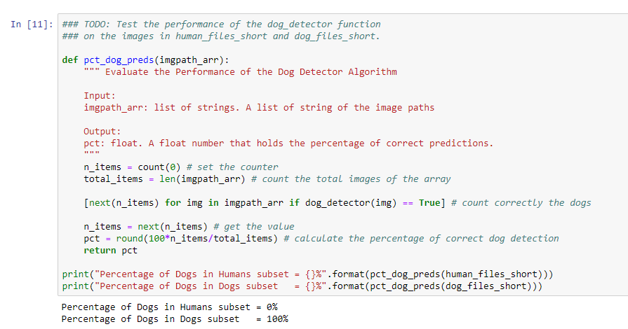
In the end, we also evaluate the model by counting the percentage of Dogs detected on the humans dataset subset and the dog dataset subset. As expected, the deep learning model detects correctly all the dogs.
Creating Your Own Vanilla Deep Learning Model
Now we will start creating a first model from scratch. And because of that we will get low accurracy. There are techniques that we will use to improve the accuracy of the network.
And how many deep layers we will add, well, depends, there is no number or magic wand that would told use, but we must be carefull of that because the more trainable layers, the more GPU time and there are also other problems like vanishing gradients that will probably you do not want to come from too soon in your vanilla model.
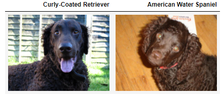
Classifying images of some breeds are challenging, for example the Retreiver and the Spaniel are very often confused by an human, and that is why deep learning comes very handy here as a feature extractor.
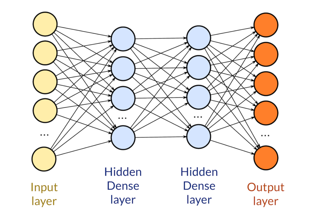
Let’s explain a little bit the inner details of the CNN
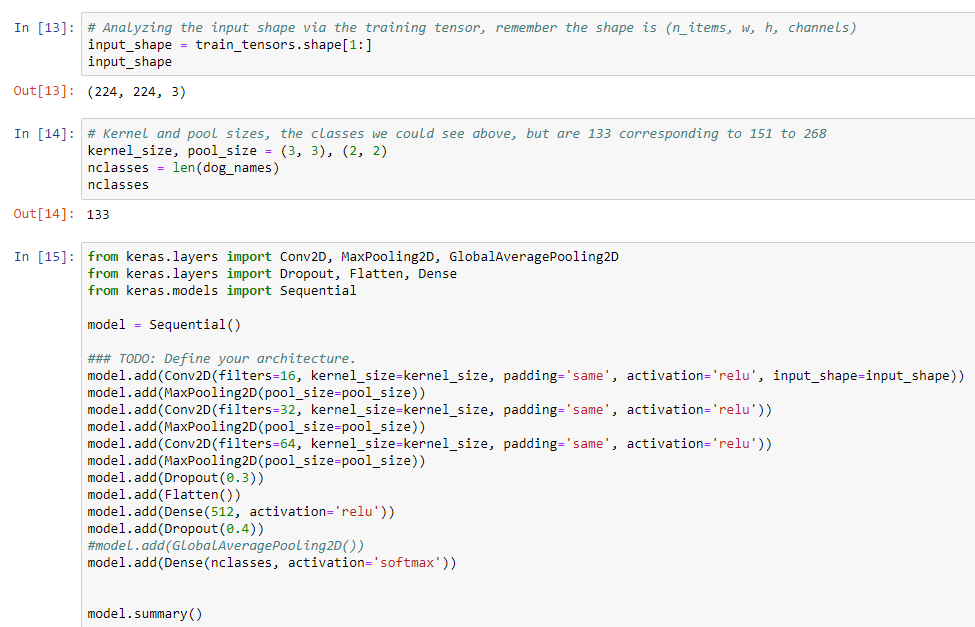
A convolution is a matrix multiplication. Concentrating on the convolution of the first layer it has 16 filters of 3×3. So we will pass all around our matrix using these 3×3 kernel over the image until the end of the image, remember, there are 16 filters. And because sometimes we could miss information of the convolution, we ensure a zero padding using ‘same’.
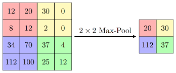
Another layer that we are using is the Max Pooling layer, this is pretty simpe to understand, it is just to get over the image with a pool or stride that will ensure to pass it matrix over the resulting image of the previous layer (Conv2D) and will get the maximum of that part, this will reduce the feature representation.
A very common layer to prevent overfitting of the training is a Dropout Layer. This layer disconnects at training time some layers in one moment to another, this will ensures that the model predict the correct features.

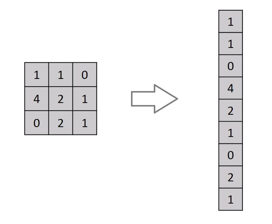
Another layer that we used is a Flatten layer, the Flatten layer is used to make my multidimensional layer linear to pass it onto a Dense layer.
Finally a Dense layer is used with a softmax activation function. Remember that these layer is responsible to make the predictions so we will need to specify the number of classes needed to detect, in this case 133.
Before training we use a method to improve the dataset, this is very often done when you are using images. Is called Data Augmentation. Basically we get an image and apply some basic transformations like skew, rotations, flips, resizing and store the images result in the memory, not the disk.
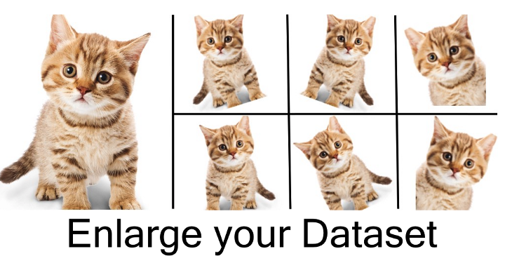
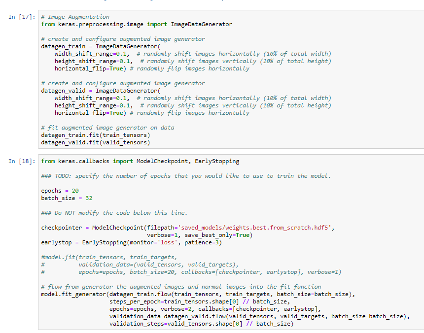
Keras has a function that implements data augmentation and also push the created images dinamically to the fit function. This function will not generate an image in the disk but in memory. If you want to see the image you have to graph the created generated images.
Finally we get a Test accuracy of 17.5837%, yes, we know is a little bit lower accuracy for a neural network, but remember, this is our vanilla implementation. So in the next section we will improve our model using a common technique when you have a small dataset.
Create a CNN to Classify Dog Breeds using Transfer Learning
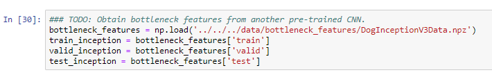
We only have 8351 image in our dataset, that is why our vanilla implementation struggles to get a good accuracy. In deep learning and the data science world, we have to feed our neural network with tons of images to make it work. Here we will use the InceptionV3 model, this is another popular architecture that won the ImageNet competition with really good acurracy. The technique implemented is called transfer learning and let us to have a small dataset and train a current pre-trained network with replacing the last layer only with our structure to make it classify our dog breeds.
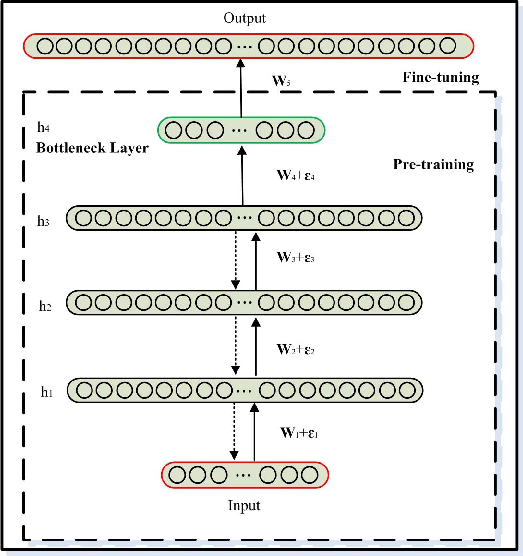
In the above figure we can see an example of a pre-trained neural network for transfer learning. The bottleneck features that we will use are the InceptionV3 features that were pre-computed by udacity and imported by loading with a numpy load function.
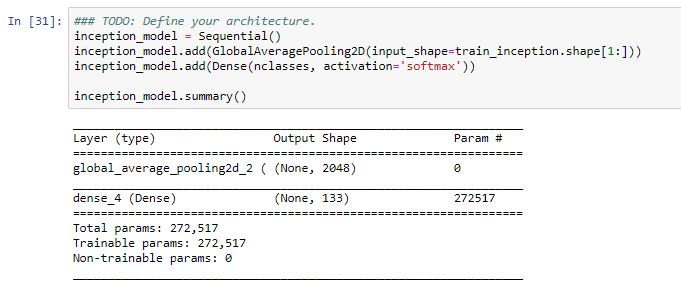
Continuing with the model architecture as seen in figure 19, we only need to add the last layers or any convolutional layers that we need; because the other parts of the model are a large neural network we will only need the last layer that is conformed of a global average pooling layer and a dense layer with the number of classes.
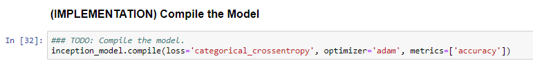
After that point we need to compile the model. We will be using categorical cross entropy because is a multiclass classification problem and the optimizer that we will use is adam.
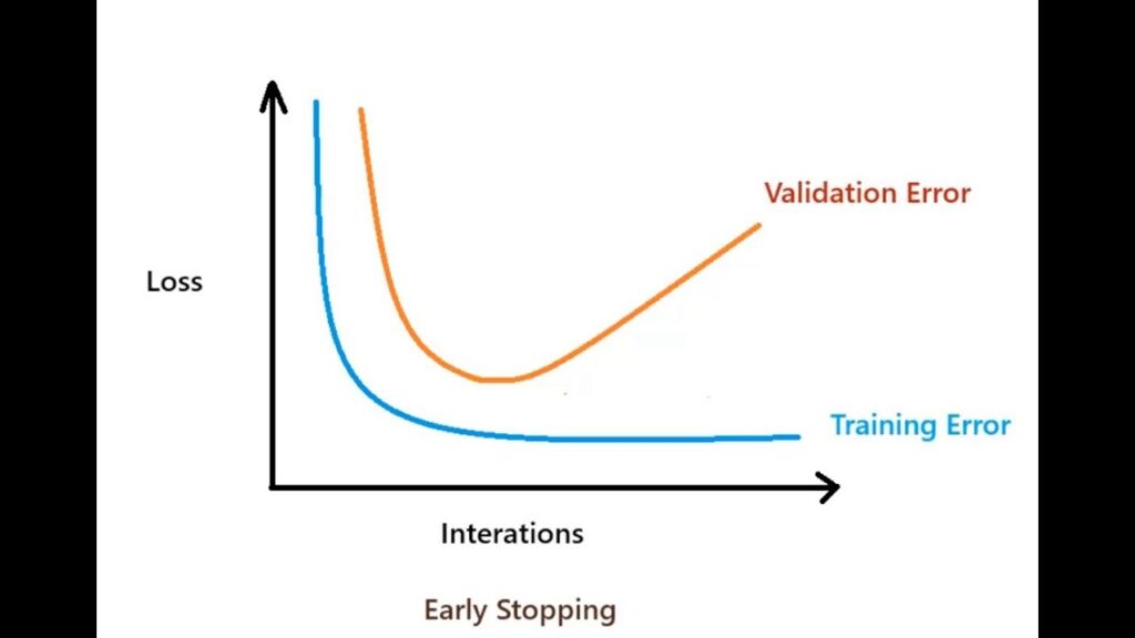
When it comes with the training part we will use a modelpoint checker, this function will save the model that attains the best validation loss. Also for improving the accuracy of the model we will use data augmentation and flow the generation of the images to the fit function of the model. On the other hand we will use a technique called early stopping to prevent overfitting and not waste time for training the model too much time if it tries to overfit.
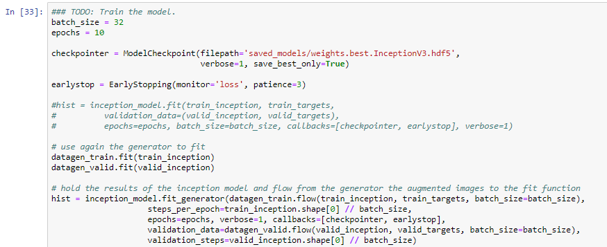
Below you will see on figure 24 the early stopping technique. If the model tries to diverge too much, the callback function will stop the training and get the best implemented training part of the model.
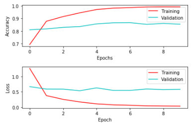
Finally we get these metrics with batches of 32 images at 10 epochs, please see the final graph to see the training and validation loss and accuracies by each epoch:
- Training Loss 0.0297
- Training accuracy 99.49%
- Validation Loss 0.5334
- Validation Accuracy 85.82%
Now we can evaluate our model with non seen data. For this we will use test targets. Hooray!, we get better results now that are better than our vanilla implementation 83%, not so bad for a first try.

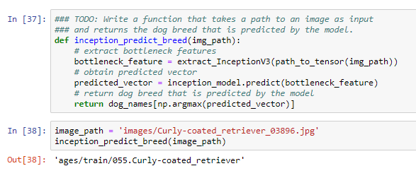
We are ready for predict dog breeds, so remember, we need to extract the tensor image and insert to our model using the predict method. Finally we will get the maximum predicted probability that will return the name of the dog from a limited dictionary.
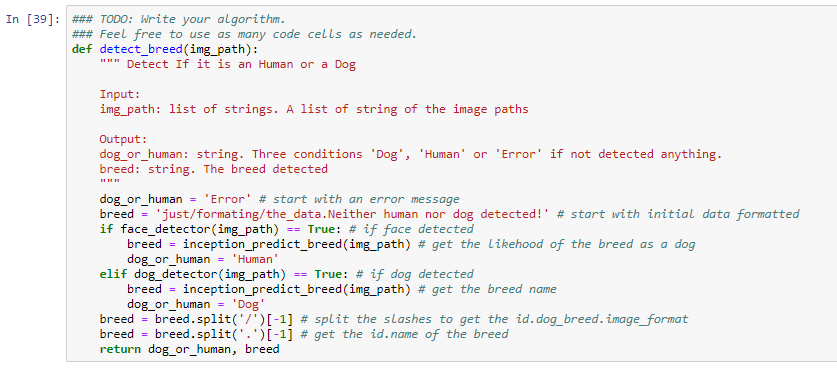
Hold on, we are finishing!. Last part is to make the algorithm to detect if there is a human, a dog or none of the others. If there is a human try to predict the breed, just for fun and if is an error display a message.
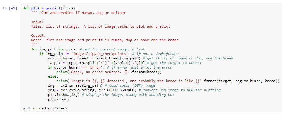
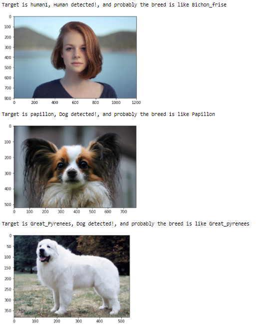
Results are by far better than our vanilla model. We must test with several images that have not seen in the dataset before to make it fair for a model prediction
Conclusion
Talking about modeling, we get accuracies of the test set of 16% with the vanilla model, 42% for the VGG16 model and 83% with the inception augmented model. We could say the model was really improved because the predictions were basically correct all the time.
Some very interesting point to me where that:
- With a few examples and a pre-trained model we could get very good predictions.
- Probably using another pre-trained models and metrics we could get better behaviors of the model
- We could experiment in a future with the other frozen layers to retrain again, but this time we only add some layers on the bottleneck
- How difficult is to construct your own model to achieve a good metric
Later we predicted from a subset of internet images if there were humans or dogs and predicted the breed of the dog… or the human, just for fun.
Transfer learning is a technique that we can use to achieve good accuracy results with small datasets and it is a fast way to get in a small amount of time a good model. The reason that gets high measurements is that we frozen previous layers and we only retrain the last layers of the new layers to make predictions on our new classes.
To improve more the accuracy of the transfer learning method we could use several modifications of this techniques (transfer learning and others) like:
- Changing the size of Dense layers
- Fine tune the new network hyperparameter like the epochs, learning rate and batch size
- Insert dropout layers to prevent overfitting
- Use different optimizers
- Use data augmentation that will get an extra boost of images to the training and improve a little the results
References
[1] OpenCV Haar-Cascades at PyImageSearch
[2] ResNet-50 model architecture and coding
[3] Popular Image Classifiers in ImageNet Competition
[4] Failure of Classification Accuracy for Imbalanced Class Distributions
Post a Comment